Guidance for Open Source 3D Reconstruction Toolbox for Gaussian Splats on AWS

Summary: This implementation guide provides an overview of the Guidance for Open Source 3D Reconstruction Toolbox for Gaussian Splats on AWS, its reference architecture and components, considerations for planning the deployment, and configuration steps for deploying the Guidance name to Amazon Web Services (AWS). This guide is intended for solution architects, business decision makers, DevOps engineers, data scientists, and cloud professionals who want to implement Guidance for Open Source 3D Reconstruction Toolbox for Gaussian Splats on AWS in their environment.

Overview

Guidance for Open Source 3D Reconstruction Toolbox for Gaussian Splats on AWS provides an end-to-end, pipeline-based solution on AWS to reconstruct 3D scenes or objects from images or video inputs. The infrastructure can be deployed with AWS Cloud Development Kit (AWS CDK) or Terraform, leveraging infrastructure-as-code.

Use cases

Once deployed, the Guidance features a full 3D reconstruction back-end system with the following customizable components or pipelines:

1. Media Ingestion: Process videos or collections of images as input
2. Image Processing: Automatic filtering, enhancement, and preparation of source imagery (for example, background removal)
3. Structure from Motion (SfM): Camera pose estimation and initial 3D point cloud generation
4. Gaussian Splat Training: Optimization of 3D Gaussian primitives to represent the scene using AI/ML
5. Export and Delivery: Generation of the final 3D asset in standard formats for easy viewing and notification by email

By deploying this Guidance, users gain access to a flexible infrastructure that handles the entire 3D reconstruction process programatically, from media upload to final 3D model delivery, while being highly modular through its componentized pipeline-based approach. This Guidance addresses the significant challenges organizations face when trying to create photorealistic 3D content—traditionally a time-consuming, expensive, and technically complex process requiring specialized skills and equipment.

Custom GS pipeline container

A Docker container image contains all of the 3D reconstruction tools for Gaussian Splatting in this project. This container has a Dockerfile, main.py, helper script files, and open source libraries under the source/container directory. When running the container in conjunction with AWS services, the source/container/src/main.py script processes each request from either the Amazon SageMaker Training Job or AWS Batch Job invoke message and saves the result to S3 upon successful completion. In order to optimize debugging, the container can be ran in LOCAL_MODE on a local computer and details can be found within the container README located at source/container/LOCAL_DEBUG_README.md.

The list of open source libraries that make this project possible include:

• NerfStudio (Apache-2.0) - Splat Training Engine
• Glomap(BSD-3-Clause) - Global SfM
• Colmap (BSD) - Incremental SfM
• OpenCV (Apache-2.0) - Video and Image Processing
• gsplat (Apache-2.0) - Splat Model
• splatfacto-w (Apache-2.0) - Splat Model
• 3DGRUT (Apache-2.0) - Gaussian Ray Tracing Model
• backgroundremover (MIT) - General Background Remover for Objects
• rembg (MIT) - Use u2net to Classify Objects and Remove/Mask them
• Attentive-Eraser (Apache-2.0) - Erase Objects in Images Using Diffusion/In-Painting
• sam2 (Apache-2.0/BSD-3-Clause) - High Quality Background Remover for Objects in Video
• SuperSplat (MIT) - Splat Editor, Compressed Splat Representation
• Gradio (Apache-2.0) - UI and Splat Viewer
• Splat-Transform MIT - CLI Tool for Splat Conversion and Transforms
• Map-Anything (Apache-2.0) - Feed Forward Transformer Model for 3D Reconstruction
• spz (MIT) - Compressed Splat Representation
• Sharp Frame Extractor (MIT) - Remove Blurry Images from Video Input

Please see repo readme for a full list of features supported!

User interface and viewer

A Gradio UI is provided in this Guidance to assist in the generation process. This UI enables users to submit gaussian splatting jobs, as well as view the generated splat in an interactive 3D viewer.

Features and benefits

This 3D reconstruction toolbox on the cloud allows customers to quickly and easily build photorealistic 3D assets from images or video using the best-in-class open source libraries that have commercial friendly licensing. This guide includes an automated end-to-end experience from deployment, submitting requests, and viewing the 3D result in a 3D web browser.

Architecture overview

This Guidance will:

• create the infrastructure required to create a Gaussian splat from a video or set of images.
• create the mechanism to run the code and perform 3D reconstruction.
• enable a user to create a 3D gaussian splat using open source tools and AWS by uploading a video (.mp4 or .mov) or images (.png or .jpg) and metadata (.json) into Amazon Simple Storage Service (Amazon S3).
• provide a 3D viewer for viewing the photo-realistic effects and performant nature of gaussian splats.

Deployment architecture diagram

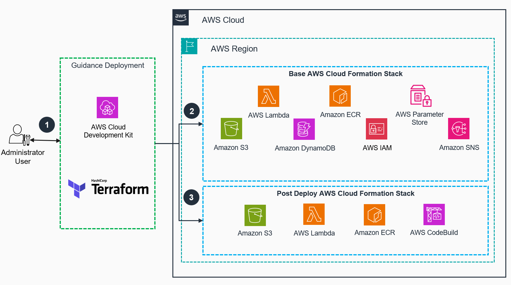
Figure 1: 3D Reconstruction Toolbox for Gaussian Splats on AWS Deployment Architecture

Deployment architecture steps

1. An administrator deploys the Guidance to an AWS account and Region using AWS Cloud Development Kit (AWS CDK) or Terraform.

2. The Base AWS CloudFormation stack to deploy will create all the AWS resources needed to host the Guidance. This includes: an Amazon Simple Storage Service (Amazon S3) bucket, AWS Lambda functions, an Amazon DynamoDB table, necessary AWS Identity and Access Management (IAM) permissions, and an Amazon Elastic Container Registry (Amazon ECR) image registry. Additionally, it includes an AWS Step Functions state machine resource ID in Parameter Store, a capability of AWS Systems Manager, and it creates an Amazon Simple Notification Service (SNS) topic.

3. Once the Base AWS Cloud Formation stack has been deployed, the Post Deploy AWS Cloud Formation stack should be deployed. That stack will build a Docker container either locally or using AWS CodeBuild, push it to the Amazon ECR registry, and also build and push the pre-processing models used during training, such as for background removal, into Amazon S3 bucket using AWS Lambda.

Architecture diagram

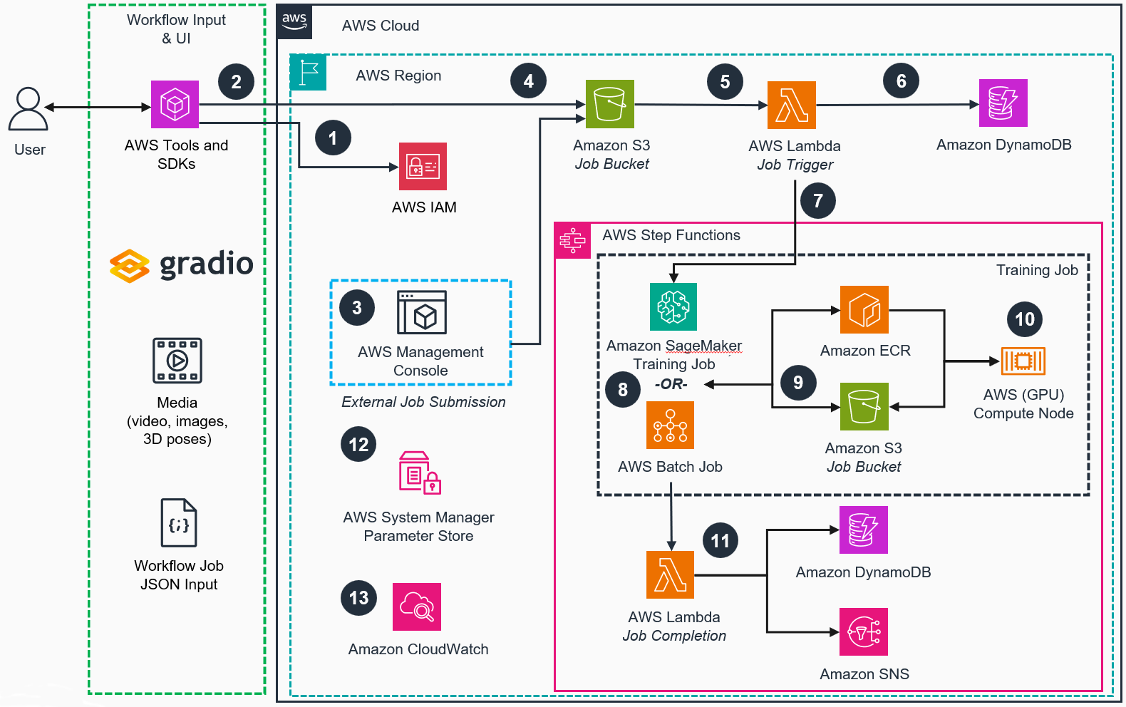
Figure 2: 3D Reconstruction Toolbox for Gaussian Splats on AWS Workflow Architecture

Architecture steps

1. The user authenticates to IAM using AWS Tools and SDKs.
2. The input is uploaded to a dedicated S3 job bucket location. This can be done using a Gradio interface and AWS Software Development Kit (AWS SDK).
3. Optionally, the Guidance supports external job submission by uploading a ‘.JSON’ job configuration file and media files into a designated S3 job bucket location.
4. The job JSON file uploaded to the S3 job bucket will trigger an Amazon SNS message that will invoke the initialization Job Trigger Lambda function.
5. The Job Trigger Lambda function will perform input validation and set appropriate variables for the Step Functions State Machine.
6. The workflow job record will be created in the DynamoDB job table.
7. The Job Trigger Lambda function will invoke Step Functions State Machine to handle the entire workflow job.
8. Based on the JSON, the process will use either an Amazon SageMaker Training Job (On-Demand) or AWS Batch Job (Spot Instance) that will be submitted synchronously using the state machine built-in wait until completion mechanism.
9. The Amazon Elastic Container Registry (ECR) container image and S3 job bucket model artifacts will be used to deploy a new container on a Graphics Processing Unit (GPU) based compute node. The compute node instance type is determined by the job JSON configuration.
10. The container will run the entire pipeline as an Amazon SageMaker training job or AWS Batch job on a GPU compute node.
11. The Job Completion Lambda function will complete the workflow job by updating the job metadata in DynamoDB and using Amazon SNS to notify the user through email upon completion.
12. The internal workflow parameters are stored in Parameter Store during deployment to decouple the Job Trigger Lambda function and the Step Function State Machine.
13. Amazon CloudWatch logs and monitors the training jobs, surfacing possible errors to the user.

AWS services in this Guidance

Security

When you build systems on AWS infrastructure, security responsibilities are shared between you and AWS. This shared responsibility model reduces your operational burden because AWS operates, manages, and controls the components including the host operating system, the virtualization layer, and the physical security of the facilities in which the services operate. For more information about AWS security, visit AWS Cloud Security.

• All data is encrypted at rest and at transit within the AWS Cloud services in this Guidance
• An Amazon S3 access logging bucket logs all access to the asset bucket
• Input validation on the job configuration will flag any misconfigurations in the json file
• Least priviledge access rights on service actions

Plan your deployment

Service quotas

Service quotas, also referred to as limits, are the maximum number of service resources or operations for your AWS account.

Quotas for AWS services in this Guidance

• Service quotas - increases can be requested through the AWS Management Console, AWS command line interface (CLI), or AWS SDKs (see Accessing Service Quotas)

• This Guidance runs either SageMaker Training Jobs or Batch Jobs which uses a Docker container to run the training. This deployment guide walks through building a custom container image that will work with SageMaker or Batch. You will be able to select between the two processing types based on the job configuration.

  • Depending on what instances you will be using to process and train on (configured during job submission, ml.g5.4xlarge is the default), you may need to adjust the SageMaker Training Jobs or EC2 quota. This will be under the SageMaker service in Service Quotas named “training job usage” or EC2 service quota named “All G and VT Spot Instance Requests”.
  • (Optional) You can optionally build and test this container locally (not running on SageMaker or Batch) on a GPU-enabled EC2 instance. If you plan to do this, increase the EC2 quota named “Running On-Demand G and VT instances” and/or “Running On-Demand P instances”, depending on the instance family you plan to use, to a desired maximum number of vCPUs for running instances of the target family. Note, this is vCPUs NOT number of instances like the SageMaker Training Jobs quota.

Cost

You are responsible for the cost of the AWS services used while running this Guidance. As of May 2025, the cost for running this Guidance with the default settings in the default AWS Region (US East 1(N. Virginia)) is approximately $73.33 per month for processing 100 requests (~$0.73 per splat generation).

We recommend creating a Budget through AWS Cost Explorer to help manage costs. Prices are subject to change. For full details, refer to the pricing webpage for each AWS service used in this Guidance.

Cost table

The following table provides a sample cost breakdown for deploying this Guidance with the default parameters in the US East (N. Virginia) Region for per month. This is based on an estimated 100 requests during a month span.

Note: Amazon SageMaker can be used instead of AWS Batch for on-demand processing, bypassing any wait queues for ~$142.33/month total

Deploy the Guidance

Prerequisites

• AWS account with IAM user or role with elevated permissions to deploy resources (Admin recommended for test accounts)
• Local computer with appropriate AWS credentials to deploy the CDK or Terraform solution
• (Optional, but recommended) Use an Amazon Elastic Compute Cloud (Amazon EC2) workstation to build and deploy the CDK or Terraform solution

  • Ensure your local computer has an SSH client (For Windows, Putty was tested)
  • Ensure your local computer has the NICE DCV client installed Windows , MacOS , or Linux
  • A CloudFormation template is given here to spin up a fresh, full-featured Ubuntu desktop
    1. Prerequisites: Before you build the EC2 workstation stack, ensure the following resources are created in your AWS account and region of choice:
       • VPC
         • Follow these instructions if you do not have one. This will be where your EC2 will live. Ensure there is a public subnet available with internet access in order to pull the GitHub repositories.
       • Keypair
         • Follow these instructions if you do not have one. This is used to remote into the EC2 desktop.
       • Security Group
         • Follow these instructions to create a security group. Enable inbound NiceDCV using TCP/UDP port 8443 and SSH using port 22. Ensure your source IP address is the resource for all entries.
         • For Inbound rules, add:
           • Custom TCP, Port range=8443, source="My IP"
           • Custom UDP, Port range=8443, source="My IP"
           • SSH, Port range=22, source="My IP"
           • If you plan on using the included Gradio user interface to submit jobs, enable the default port so you can access the app through your local browser.
             • Custom TCP, Port range=7860, source="My IP"
         • Record the security group Id for later
    2. Download the deep-learning-ubuntu-desktop.yaml file locally from the repo linked above
    3. Open the AWS Console and navigate to the CloudFormation console
    4. Select 'Create stack' -> 'With new resources'
    5. On `Create Stack` page, select:
       • Choose an existing template
       • Choose Upload a template file
       • Select the deep-learning-ubuntu-desktop.yaml file downloaded earlier
    6. On Specify stack details page, leave default values except for the following:
       • Stack Name: YOUR-CHOICE
       • AWSUbuntuAMIType: UbuntuPro2204LTS
       • DesktopAccessCIDR: YOUR-PUBLIC-IP-ADDRESS/32
       • DesktopInstanceType: g5.2xlarge
       • DesktopSecurityGroupId: SG-ID-FROM-ABOVE
       • DesktopVpcId: VPC-ID-FROM-ABOVE
       • DesktopVpcSubnetId: YOUR-PUBLIC-SUBNET-ID
       • KeyName: KEYNAME-FROM-ABOVE
       • (optional) S3Bucket: S3-BUCKET-WITH-CODE
    7. Submit and monitor the stack creation in the CloudFormation console
    8. On successful building of the stack, navigate to the EC2 console in the account and region the deployed stack is in
    9. Locate the instance just created using the `Stack Name` entered above, select the instance, and select Actions->Security->Modify IAM Role
    10. Record the current IAM role name
    11. Navigate to the IAM Console in a separate browser tab or window
    12. Under `Roles`, search for the role using the IAM role name identified above
    13. Select the role by clicking on its name
    14. In the permissions policies table, select Add permissions->Attach policies:
        • Attach the following AWS managed policies to the role
          • AmazonEC2ContainerRegistryFullAccess
          • AmazonS3FullAccess
          • AmazonSSMManagedInstanceCore
          • AWSCloudFormationFullAccess
          • IAMFullAccess
    15. SSH into the workstation using the EC2 public IP (found in the EC2 console), security group, and SSH terminal
    16. Once connected to the EC2 workstation, perform the following commands to update the OS and password

                  
                  sudo apt update
                  sudo passwd ubuntu
                  
                  

    17. The EC2 will reboot automatically while updating is being performed in the background
    18. The EC2 setup is complete once the message echo 'NICE DCV server is enabled!' is shown when performing the following command

                  
                  tail /var/log/cloud-init-output.log
                  
                  

    19. Once the EC2 has the enabled NICE DCV message, use the NICE DCV client, EC2 public IP address, username 'ubuntu' and Ubuntu password set earlier to remotely connect to the EC2 instance.
    20. Be sure to not upgrade the OS (even when prompted) as it will break critical packages. Only choose to enable security updates.
    21. Open the Visual Code program in the EC2 instance by locating it in the Application library

• Install and configure the AWS CLI (if not using the recommended EC2 deployment below)

  • Install or update the latest version of the AWS CLI

  • Set up the AWS CLI - create configuration and set up credentials

• Install Git (if not using the recommended EC2 deployment below)

• Docker installed (if not using the recommended EC2 deployment below or AWS CodeBuild option)
  • N.B. buildx is also required. For Windows and macOS buildx is included in Docker Desktop
  • Docker is required to build the container image that is used for training the splat. This will require at least 20GB of empty disk space on your deployment machine.

    Note: If building on Windows or MacOS and receive the below error, set the number of logical processors to 1. Also, it is recommended to use the EC2 Ubuntu deployment method or CodeBuild option below to mitigate this error.

      #17 [13/28] RUN pip install --no-cache-dir -r ./requirements_2.txt
      #17 2.026 Processing ./diff-gaussian-rasterization
      #17 2.029   Preparing metadata (setup.py): started
      #17 8.350   Preparing metadata (setup.py): finished with status 'done'
      #17 8.365 Processing ./diff-surfel-rasterization
      #17 8.367   Preparing metadata (setup.py): started
      #17 12.41   Preparing metadata (setup.py): finished with status 'done'
      #17 12.42 Building wheels for collected packages: diff-gaussian-rasterization, diff-surfel-rasterization
      #17 12.42   Building wheel for diff-gaussian-rasterization (setup.py): started
      ERROR: failed to receive status: rpc error: code = Unavailable desc = error reading from server: EOF
    

• (Optional) if using VSCode and using the Terraform deployment, the HashiCorp Terraform extension is helpful

• Visit clone a repository for instructions. Clone this repository locally.

    git clone https://github.com/aws-solutions-library-samples/guidance-for-open-source-3d-reconstruction-toolbox-for-gaussian-splats-on-aws.git
  

• Download and install Node Package Manager (NPM) if not already on your system. The LTS version is recommended.

  • For Ubuntu EC2

      sudo apt update
      sudo apt install npm nodejs -y
      sudo chown -R $USER PATH-TO-THIS-REPO
      sudo npm install -g n
      sudo n stable
    

  • For Windows/MacOS

      npm install -g npm@latest
    

• Confirm authenticated as the correct IAM principal and in the correct AWS account (see get-caller-identity for more info).

    aws sts get-caller-identity
  

• Set the AWS Region, replacing the Region below with your deployed region
  • Windows

      set AWS_REGION=us-east-1
    

  • Linux/Mac

      export AWS_REGION=us-east-1
    

Deployment process overview

Before you launch the Guidance, review the cost, architecture, security, and other considerations discussed in this guide. Follow the step-by-step instructions in this section to configure and deploy the Guidance into your account.

Time to deploy: Approximately 60 minutes

[OPTION #1: CDK instructions] Deploy backend infrastructure

1. Download and install Node Package Manager (NPM) if not already on your system. The LTS version is recommended.

   For EC2 Ubuntu, it might be necessary to add sudo privilages to the below command

    npm install -g npm@latest
   

2. Install the latest CDK toolkit (see AWS CDK Toolkit for more info). Check the version to confirm the installation was successful.

   For EC2 Ubuntu, it might be necessary to add sudo privilages to the below command

    npm install -g aws-cdk@latest
   

   Once installed, the following command will confirm installation was successful.

    cdk --version
   

3. From the project root, navigate to the deployment/cdk/ folder.

4. Open config.json and enter values for the following fields:
   • accountId - target 12-digit AWS account number
   • region - target AWS region (e.g. us-west-2)
   • s3TriggerKey - S3 name/key to use for json job submissions
   • adminEmail - valid email address used to create a user for the SNS email notifications
   • maintainS3ObjectsOnStackDeletion - whether to keep the S3 objects upon stack deletion or not
   • enableCodeBuildContainerBuild - whether to build the container on the cloud or locally

5. Create a virtual environment.

   • For Windows

     Download and install the latest Python version

     Replace PATH-TO-PYTHON-VERSION-EXE with your version and path to Python (e.g. virtualenv --python C:/Python312/python.exe 3dgs-env)

       virtualenv --python PATH-TO-PYTHON-VERSION-EXE 3dgs-env
       .\3dgs-env\Scripts\activate
     

   • For macOS/Linux

     For Ubuntu, you may need to install virtualenv using sudo apt install python3-virtualenv -y

     Replace PATH-TO-PYTHON-VERSION-EXE with your version and path to Python (e.g. virtualenv --python /usr/bin/python3 3dgs-env)

       virtualenv --python PATH-TO-PYTHON-VERSION-BINARY 3dgs-env
       source 3dgs-env/bin/activate
     

6. Install project dependencies.

    pip install -r requirements.txt
   

   Note: The next few steps will deploy resources. You can use aws sts get-caller-identity to confirm your IAM principal and AWS account before proceeding.

7. Bootstrap your environment, replacing the AWS account ID and Region below.

    cdk bootstrap aws://101010101010/us-east-1
   

8. Deploy Infrastructure Stack.

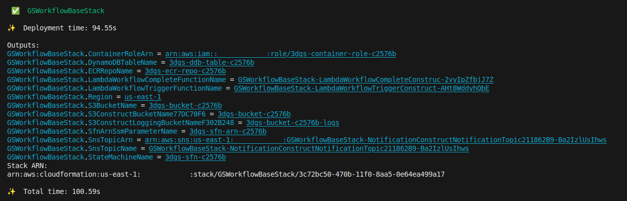
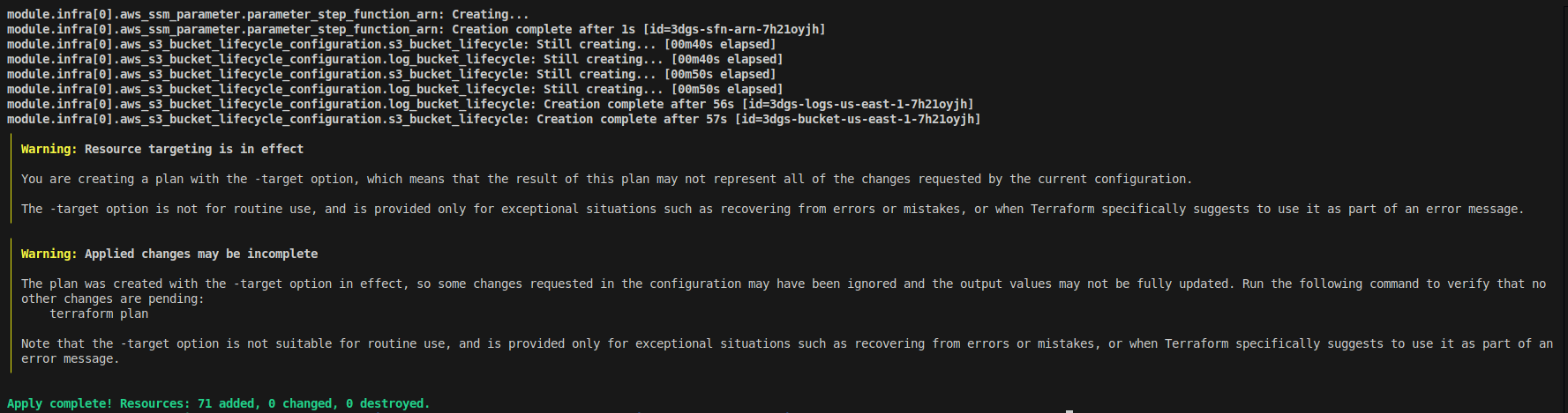
    cdk deploy GSWorkflowBaseStack --require-approval never --outputs-file outputs.json --exclusively
   

   NOTE: To view the created resource names, you can view them in CloudFormation console under Outputs, or in deployment/cdk/outputs.json

   

   Figure 3: AWS CDK Base Stack Output
9. Deploy Post Deployment Stack.

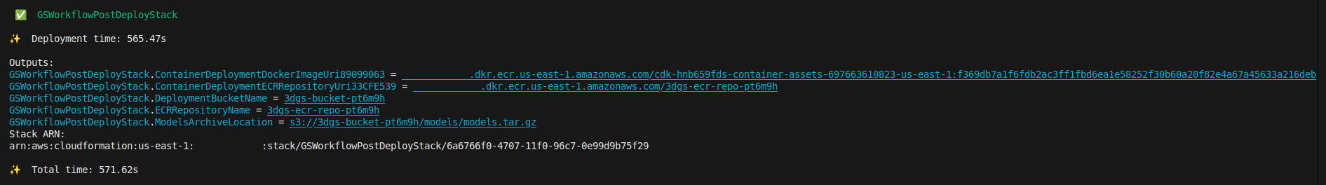
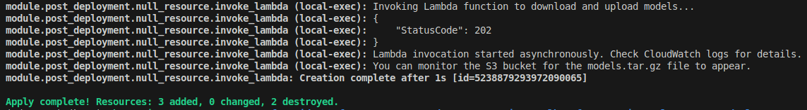
    cdk deploy GSWorkflowPostDeployStack --require-approval never --exclusively
   

   NOTE: The project take up to 2 hours to build the container and deploy. See below for Amazon SNS Notification details.

   

   Figure 4: AWS CDK Post Deploy Stack Output

   NOTE: If CodeBuild was enabled in the config.json file, execute the following command to check the status of the build.

    python check_build_status.py
   

    Status: IN_PROGRESS | Phase: BUILD | Elapsed: 0m 0s
    Status: IN_PROGRESS | Phase: BUILD | Elapsed: 0m 30s
    ...
    Status: IN_PROGRESS | Phase: POST_BUILD | Elapsed: 102m 58s
    Status: IN_PROGRESS | Phase: POST_BUILD | Elapsed: 103m 28s
    Status: SUCCEEDED | Phase: COMPLETED | Elapsed: 103m 59s
   
    ✅ Build completed successfully!
    Image: 3dgs-ecr-repo-******:latest
    Total time: 103m 59s
   

[OPTION #2: Terraform instructions] Deploy backend infrastructure

1. Install Terraform (Terraform commonly looks for AWS credentials in a shared credentials file like the one created by the AWS CLI configuration or environment variables; see AWS Provider for more info)

2. From the project root, navigate to the deployment/terraform/ folder.

3. Open terraform.tfvars and enter values for the following fields:
   • account_id - target 12-digit AWS account number
   • region - target AWS region (e.g. us-west-2)
   • admin_email - valid email address used to create a user for the SNS email notification
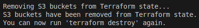
   • maintain_s3_objects_on_stack_deletion - whether to keep the S3 objects upon stack deletion or not
   • enable_code_build_container_build - whether to build the container on the cloud or locally
   • deployment_phase - used to select the deployment phase (“base” or “post”) – No need to change this directly, use the terraform -var deployment_phase flag to set

   Note: The next few steps deploys resources. You can use aws sts get-caller-identity to confirm your IAM principal and AWS account before proceeding.

4. Initialize Terraform.

    terraform init
   

5. Deploy the Terraform base environment.

    terraform apply -var "deployment_phase=base" -var-file=terraform.tfvars -target=module.infra -auto-approve
   

   • Scrolling up will reveal the created terraform execution plan which lists the resources to be created.

   NOTE: To view the created resource names, you can view them in CloudFormation console under Outputs, or in deployment/terraform/outputs.json

   

   Figure 5: Terraform Base Stack Output

6. Deploy the Terraform post deployment environment.

    terraform apply -var "deployment_phase=post" -var-file=terraform.tfvars -auto-approve
   

   NOTE: The project takes approximately an hour to build the container and deploy

   

   Figure 6: Terraform Post Deploy Stack Output

   NOTE: If CodeBuild was enabled in the terraform.tfvars file, execute the following command to check the status of the build.

    python check_build_status.py
   

    Status: IN_PROGRESS | Phase: BUILD | Elapsed: 0m 0s
    Status: IN_PROGRESS | Phase: BUILD | Elapsed: 0m 30s
    ...
    Status: IN_PROGRESS | Phase: POST_BUILD | Elapsed: 102m 58s
    Status: IN_PROGRESS | Phase: POST_BUILD | Elapsed: 103m 28s
    Status: SUCCEEDED | Phase: COMPLETED | Elapsed: 103m 59s
   
    ✅ Build completed successfully!
    Image: 3dgs-ecr-repo-******:latest
    Total time: 103m 59s
   

Post deployment requirements

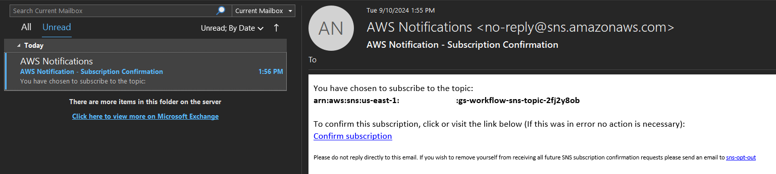
• After deployment, the admin email provided in the deployment configuration will receive an email subscription notification.

  

  Figure 7: SNS Subscription Email for jobs
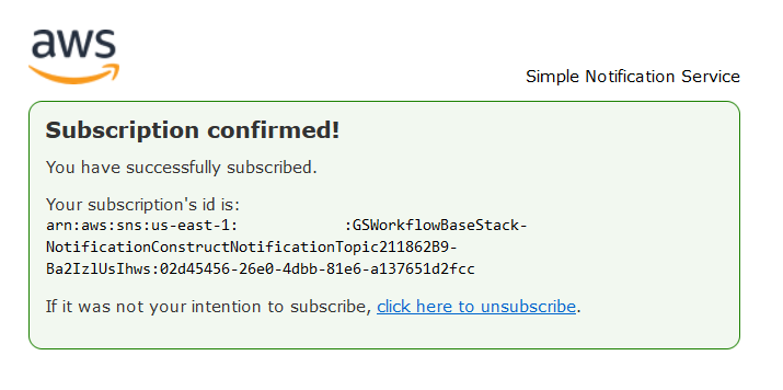
• Please enable notifications by clicking on the link in the email.

  

  Figure 8: SNS Subscription Confirmation

Submitting a job

Job submission options

To generate a splat, the backend requires a video or .zip of images and a unique metadata (.json) file to be uploaded to Amazon S3. A sample video can be used to immediately test the solution located at assets/input/BenchMelb.mov

For all options below, be sure to fill in the appropriate options and confirm you are authenticated with AWS. The default options will work for videos orbitting an object.

OPTION A. User interface with S3 library browser and 3D viewer

• A Gradio interface is included in this repo at source/Gradio/. Please follow the directions below to use it:
  • Open a console/command window of a machine that has the repo deployed
  • Change directories to the repo under the source/Gradio/ directory
  • Enter the following commands

      python -m venv venv
      source venv/bin/activate # On Windows, use: venv\Scripts\activate
      pip install -r requirements.txt
    

  • Configure the application - configure the Gradio Application to use the created bucket:
    • Open generate_splat_gradio.py in a text editor
    • Input the S3 bucket name into the self.s3_bucket = "" field
    • Save the file and exit
  • Authenticate with AWS

    • Confirm authenticated as the correct IAM principal and in the correct AWS account (see get-caller-identity for more info).

        aws sts get-caller-identity
      

  • Start the Gradio interface:

      cd source/Gradio
      python generate_splat_gradio.py
    

  • Open your web browser and navigate to the URL displayed in the terminal (typically http://0.0.0.0:7860 or use the local or public IP of the machine running the above script)

    

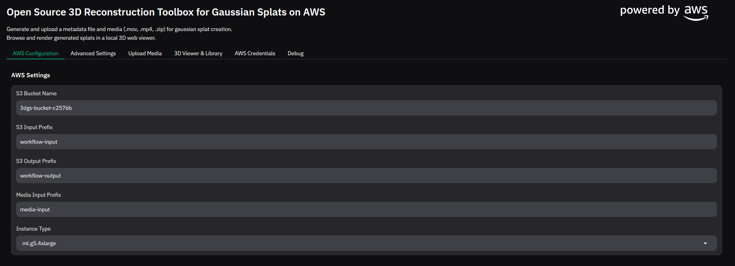
    Figure 9: Gradio App: AWS Configuration
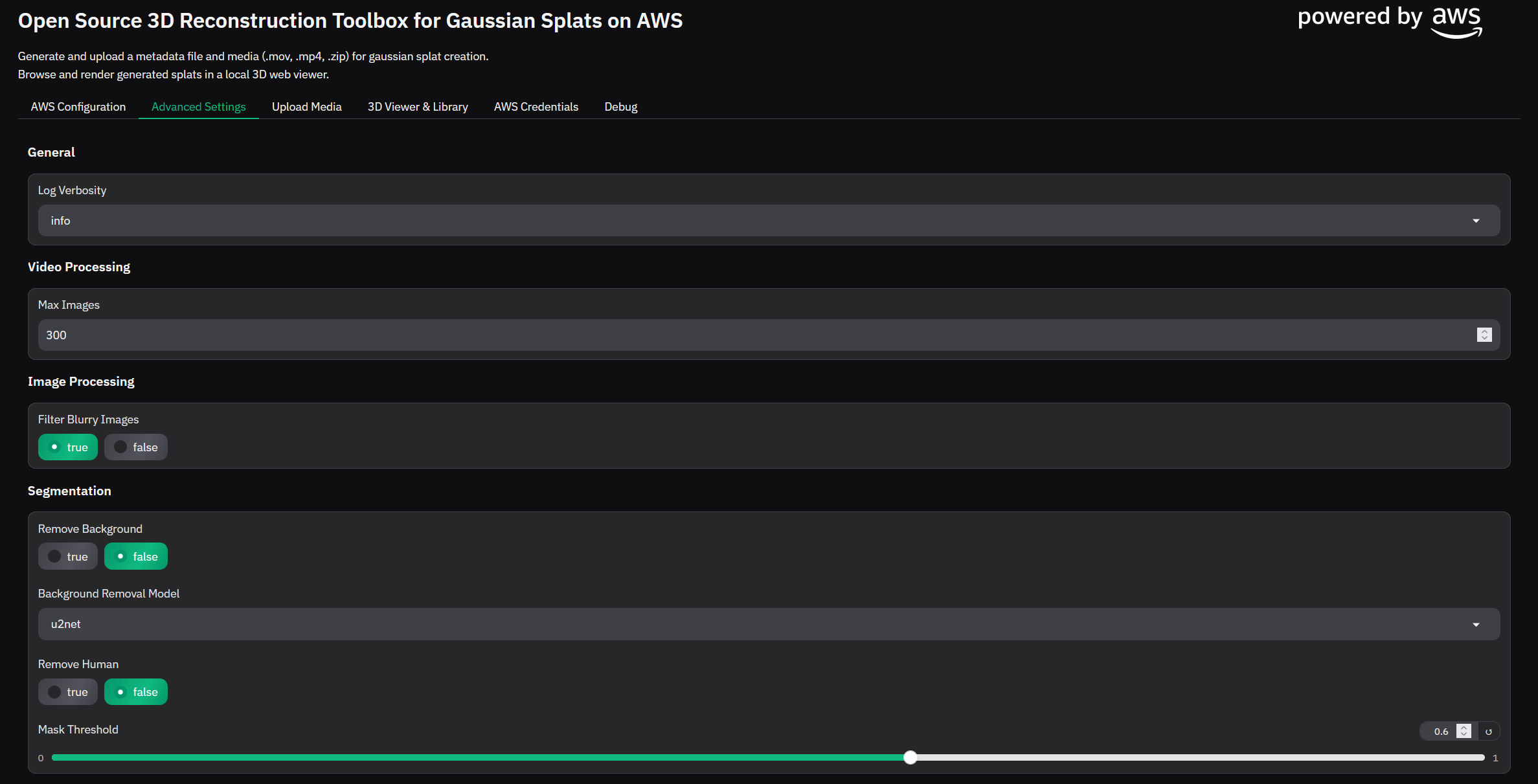
  • Navigate to the Advanced Settings tab in the app and configure the job accordingly (The default settings will work for a video with the camera orbitting an object)

    

    Figure 10: Gradio App: Job Settings
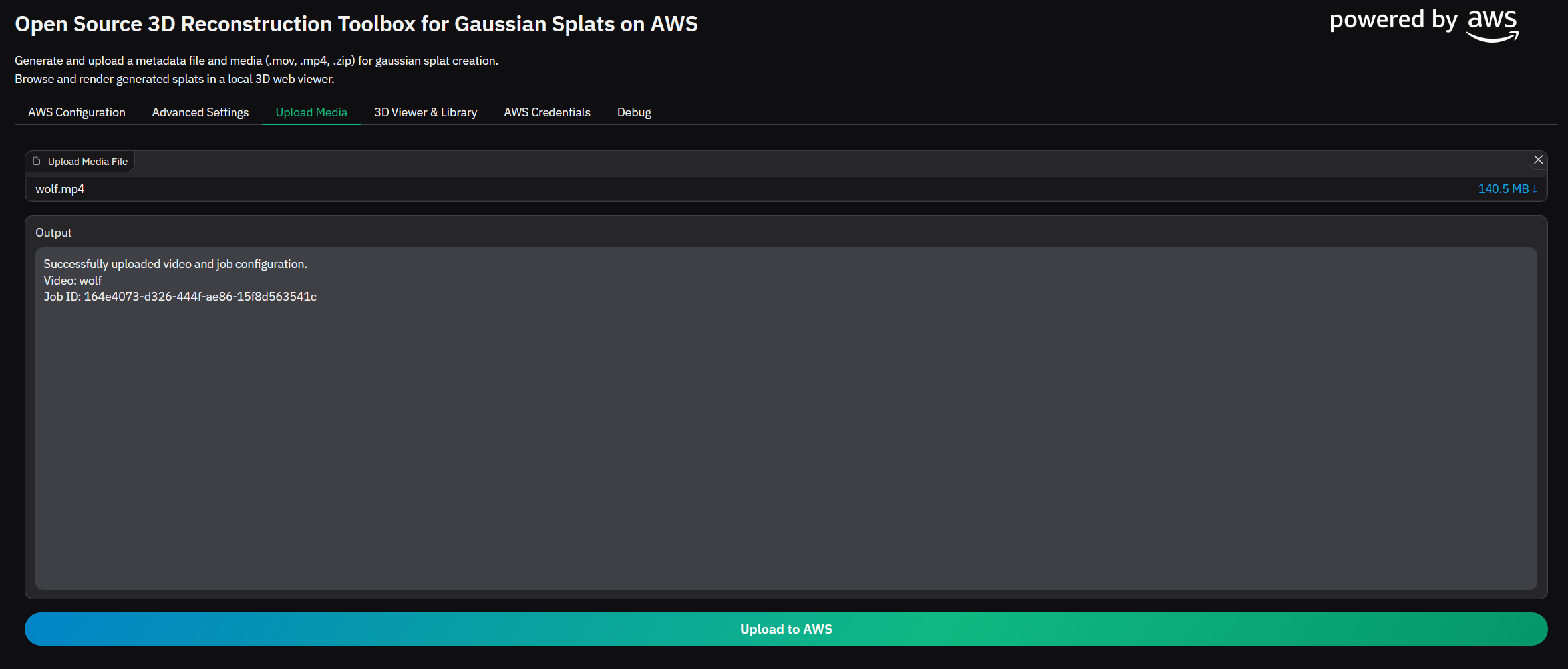
  • Navigate to the Upload Media tab in the app, input the media, then submit the job to AWS

    

    Figure 11: Gradio App: Job Submission

OPTION B. Python script and S3 upload

Follow the doc located at source/readme.md to submit jobs to the toolbox by using a Python script or AWS Console

• Use the source/generate_splat.py file to submit the artifacts and upload the media and json metafile directly into the S3 bucket.
• The metadata file can be created manually following the structure documented above or created automatically and submitted using source/generate-splat.py.
• The media and metadata (job) file can be uploaded directly into S3 to trigger the workflow using external processes or manually.

Understanding the configuration and capabilities

This Guidance is built with a variety of open source tools that can be used for various use cases. Because of this, many options are contained in this Guidance. For a high-level overview of each option and its applicability, please see the Understanding the Configuration Guide.

Monitoring a job

The training progress can be monitored a few different ways:

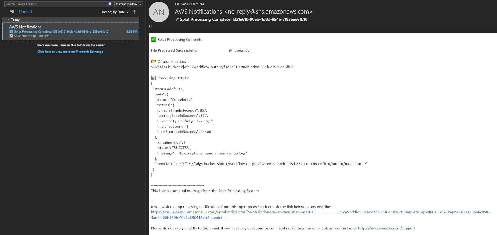
• An SNS notification will be sent once the 3D reconstruction is complete (usually 20-80 min depending on the model, quality, or time constraints)

  

  Figure 15: Job successful completion email notification using SNS

  

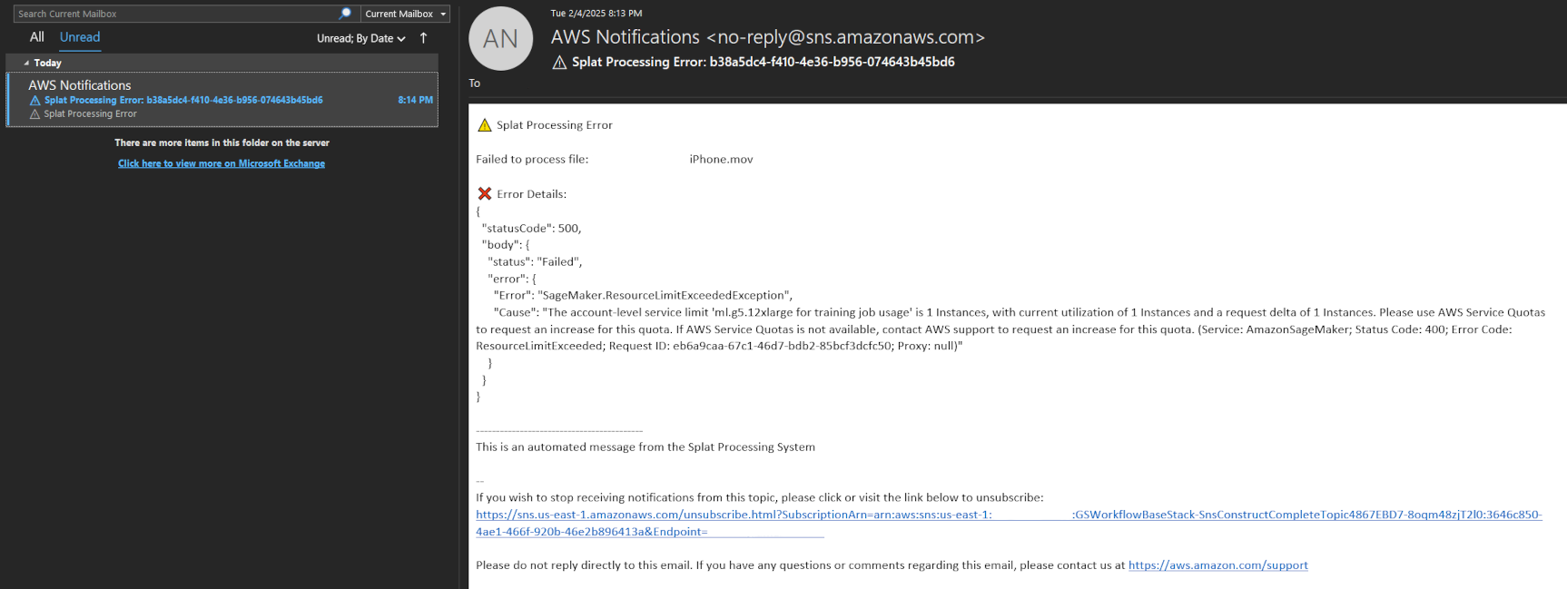
  Figure 16: Job error notification using SNS
• Gradio Interface
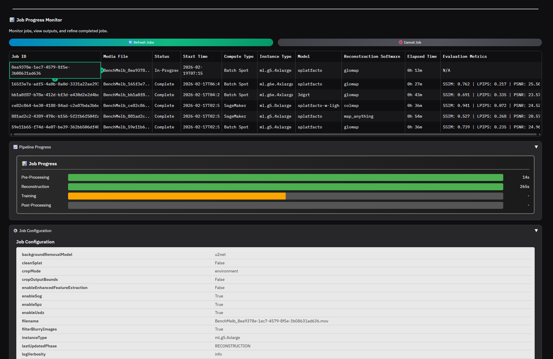
  • Jobs can be monitored in the Gradio under on the Job Monitor & Viewer tab.
  • Job progress can be observed by selecting the job in the job table and viewing the Pipeline Progress section of the UI.

  

  Figure 17: Monitor Job Status
• SageMaker
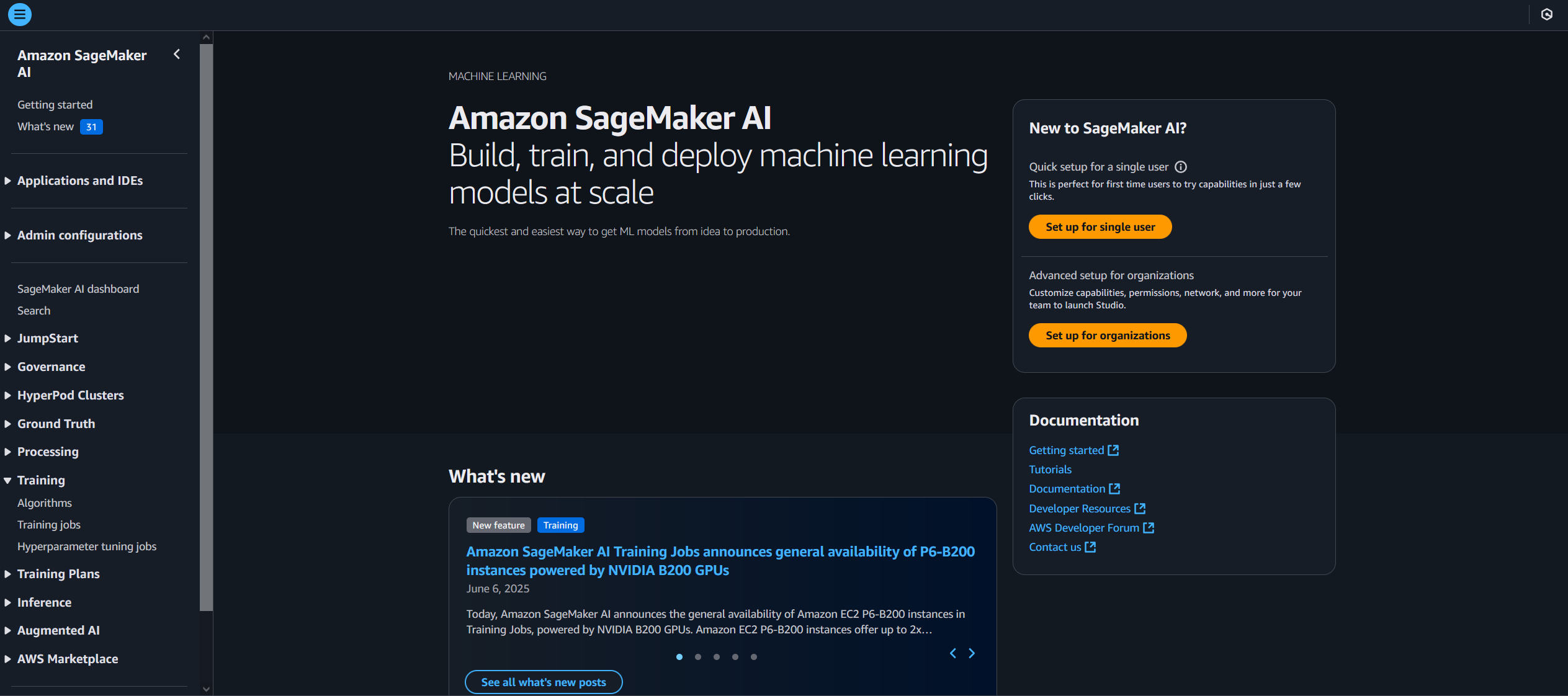
  • Using the AWS Management Console, navigate to SageMaker -> Training -> Training Jobs.

    

    Figure 18: Amazon SageMaker Training Jobs Selection
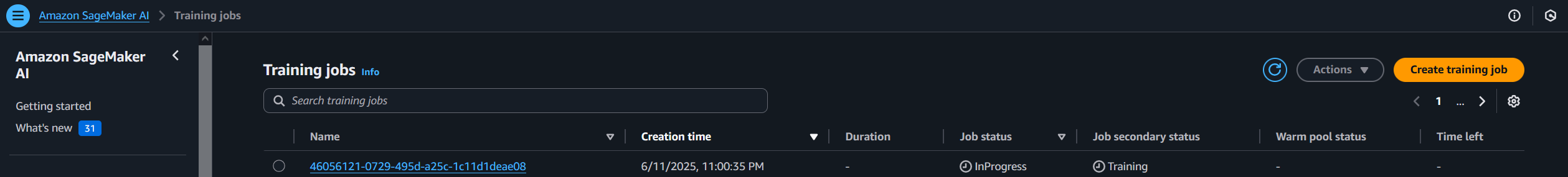
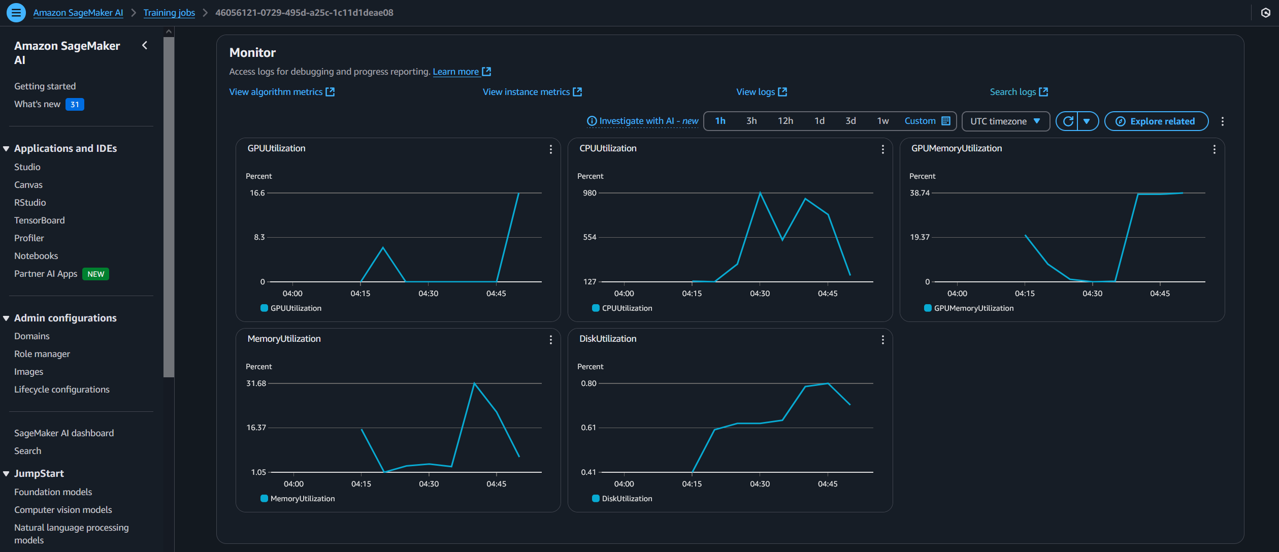
  • Enter the uuid in the search bar, and click on the entry to view status and monitor metrics/logs.

    

    Figure 19: Amazon SageMaker Training Job Status

    

    Figure 20: Amazon SageMaker Training Job Monitoring
• Batch
  • Using the AWS Management Console, navigate to Batch -> Jobs.
  • Enter the uuid in the search bar, and click on the entry to view status and monitor metrics/logs.
• Step Functions
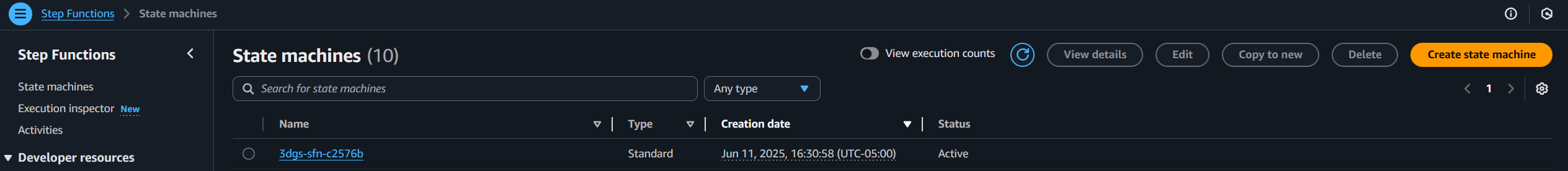
  • Using the AWS Management Console, navigate to Step Functions -> State Machines.

    

    Figure 21: AWS Step Functions State Machine Selection
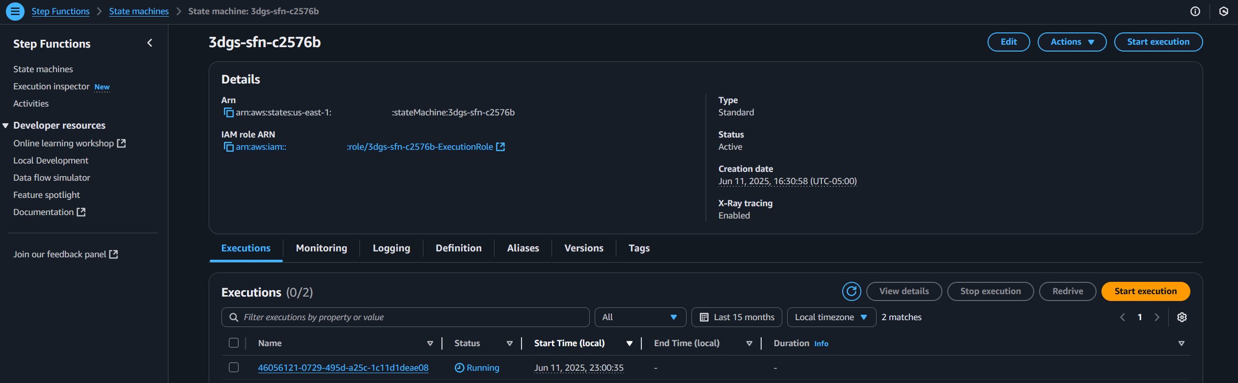
  • Enter the identifier found in outputs.json in the search bar, and click the entry to view status and monitor the state of the workflow.

    

    Figure 22: AWS Step Functions State Machine Job Detail
• CloudWatch
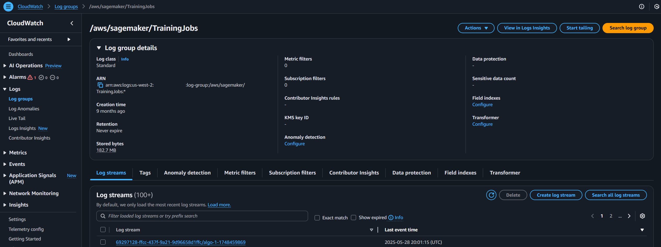
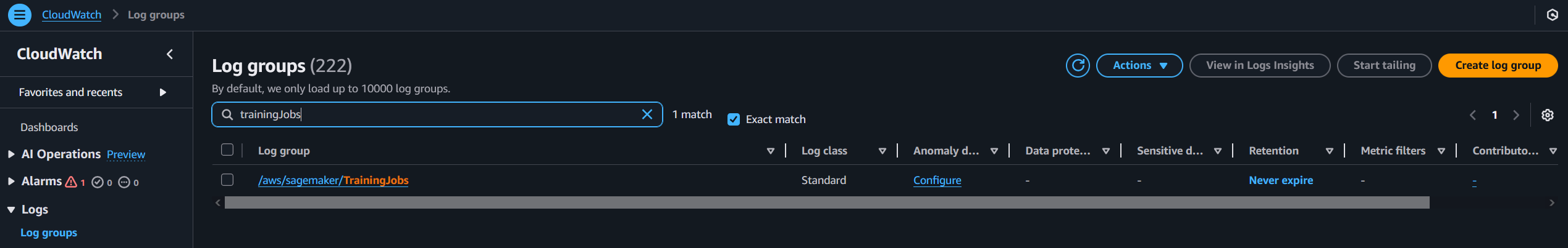
  • Using the AWS Management Console, navigate to CloudWatch -> Log Groups.

    

    Figure 23: Amazon CloudWatch Log Group
  • If the job was for SageMaker, enter /aws/sagemaker/TrainingJobs in the search bar, and click on the log group. Enter the uuid in the log stream search bar to inspect the log

    

    Figure 24: Amazon CloudWatch Training Logs
  • Otherwise enter /aws/batch/job in the search bar, and click on the log group. Enter the uuid in the log stream search bar to inspect the log

Viewing the job result

After training has completed on submitted media and an SNS email has been received, the splat result can be viewed in the Gradio user interface (see Job submission options, Option A. to launch). Once the Gradio app has been launched:

Note: The output files can be directly downloaded from S3 at {bucket}/workflow_output/{uuid}/

1. Navigate to the browser, enter the local IP of the machine you launched the Gradio app on (either the EC2 instance or host machine), and port for the app (e.g. http://01.23.456.789:7860)

   

   Figure 25: Gradio Application
2. Inside the Gradio app, navigate to the Job Monitor & Viewer tab

   

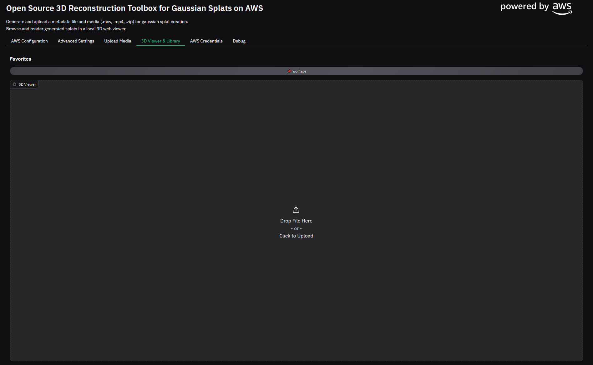
   Figure 26: 3D Viewer & Library
3. There is a sample splat located at source/Gradio/favorites/benchmelb.spz and can be viewed by clicking on the favorite button titled “benchmelb.spz”.

   

   Figure 27: Viewing Local 3D Objects
4. To select and view items from S3, click “Refresh Jobs”, and the table should populate with completed items in S3. Select an item (row) you would like to view and a job details window should pop up.

   

   Figure 28: Refreshing Table Items
5. After selecting the job, there are either two actions that will occur based on the status of the job. If the job is still running, a job progress meter can be seen.

   

   Figure 29: Monitor Job Status
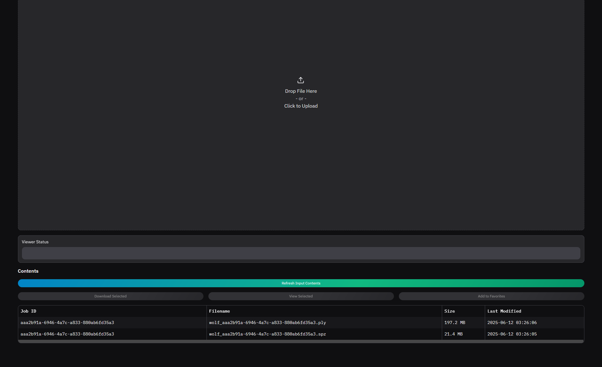
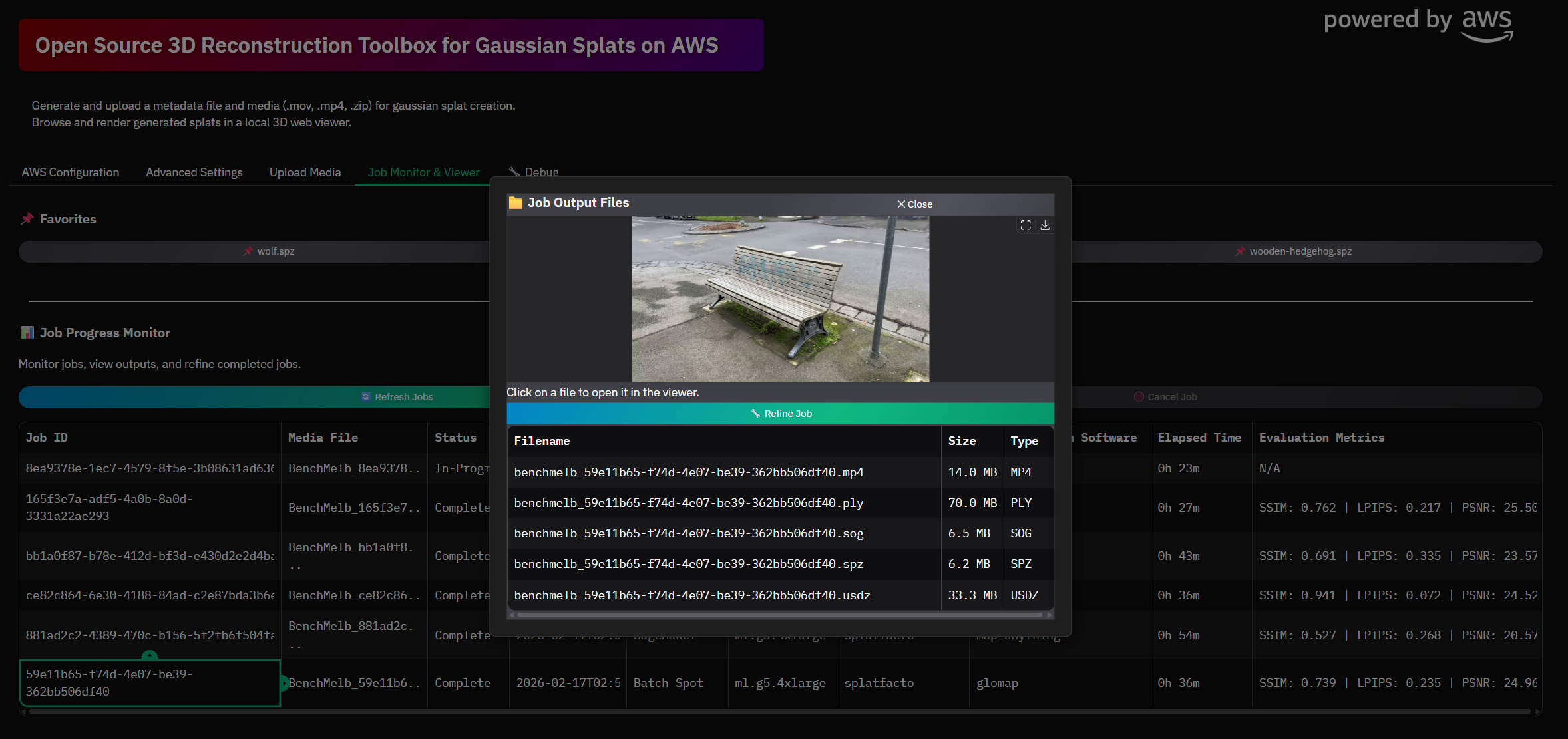
6. If the selected job is complete, the job output files will be shown in a pop up window.

   

   Figure 30: Viewing Output Files
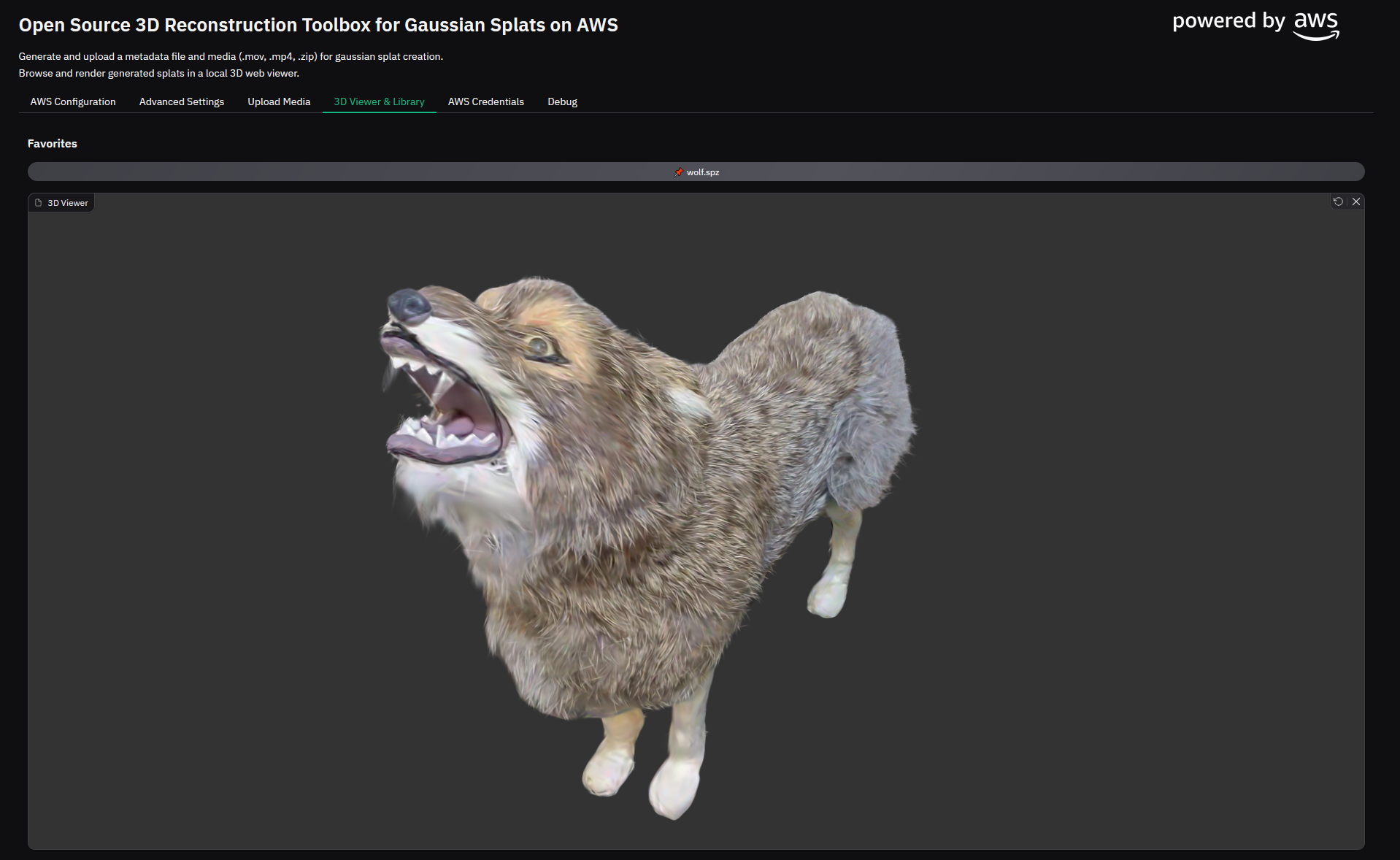
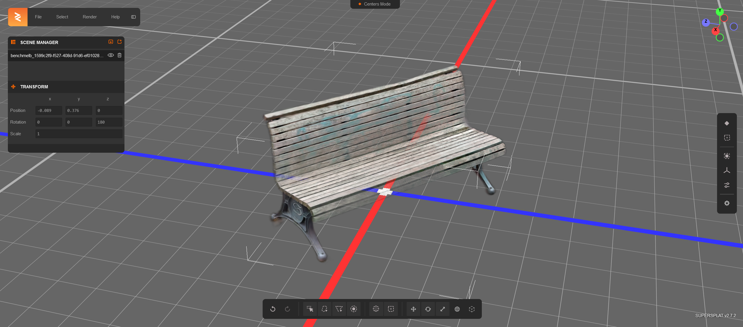
7. The splat or output video can be inspected in the 3D Viewer.

   

   Figure 31: Viewing Splats
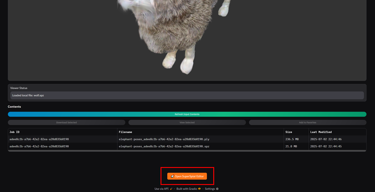
8. If you would like to edit the splat, first download it following the above step, navigate to the bottom of the 3D Viewer/Library tab and launch the SuperSplat viewer by clicking on the button. This will open up the editor in a different browser tab and allow you to drag-and-drop the downloaded splat into the editor. At the time of authoring this, the .spz format was not supported by the SuperSplat editor, but you can use the .ply file instead.

   

   Figure 32: Launching the SuperSplat Editor

   

   Figure 33: Editing Splats with SuperSplat

Tips

General

• Sample un-touched splat outputs are located in the repo at source/Gradio/favorites
• The default settings will enable you to process a video that has the camera orbiting an object. Use the assets/input/BenchMelb.mov sample as an example of capturing objects using video.
• SAM2 segmentation only works on video input, otherwise use u2net

SfM Convergence

There is a possibility that your input media is not sufficient enough to reconstruct the scene. This will cause the camera pose estimation process to not converge. This typically occurs when:

1. Image Quality Issues:
   • Insufficient overlap between consecutive frames
   • Motion blur in images
   • Poor lighting conditions
   • Low image resolution
2. Scene Characteristics:
   • Not enough distinctive features in the scene
   • Highly reflective or transparent surfaces
   • Uniform/textureless areas
   • Dynamic objects or movement in scene
3. Camera Motion:
   • Too rapid camera movement
   • Large gaps in viewpoints
   • Irregular camera paths

Additional Guidance

More guidance can be found in the Understanding the Configuration Guide and Use Case Settings Guide.

Uninstall the Guidance

Note: Be aware that this will also delete any generated assets in the S3 bucket as well, if not following directions below:

1. If not already done, delete the EC2 instance and associated resources (IAM role, key pair, security group) used to run the container script.
2. Delete the backend.
   • For Terraform:
     • Navigate to deployment/terraform
     • If you would like to keep your S3 assets, issue this command:

         sed -i 's/\r$//' ./orphan_s3.sh
         chmod +x orphan_s3.sh
         ./orphan_s3.sh
       

       

       Figure 34: Orphan S3 Bucket from Stack

       
       

     • Then, issue the destroy command:

         terraform destroy
       

       

       Figure 35: Destroy Terraform Resources

       
       

   • For CDK:
     • Navigate to deployment/cdk and issue the destroy command.
     • To destroy all resources

         cdk destroy --all -c destroy=true
       

     • To destroy individual stacks

         cdk destroy GSWorkflowBaseStack -c destroy=true
       

         cdk destroy GSWorkflowPostDeployStack -c destroy=true
       

     • Successful deletion output

          ✅  GSWorkflowBaseStack: destroyed
          ✅  GSWorkflowPostDeployStack: destroyed
       

Related resources

• Gaussian Splatting pipeline for AWS Deadline Cloud
• Building a Digital Twin with Photogrammetry and AWS IoT TwinMaker
• Photogrammetry reconstruction with 3Dflow on AWS

Contributors

• Eric Cornwell, Sr. Spatial SA
• Dario Macagnano, Sr. Worldwide Physical AI SA
• Stanford Lee, Technical Account Manager
• Daniel Zilberman, Sr. SA AWS Technical Guidances

Notices

Customers are responsible for making their own independent assessment of the information in this document. This document: (a) is for informational purposes only, (b) represents AWS current product offerings and practices, which are subject to change without notice, and (c) does not create any commitments or assurances from AWS and its affiliates, suppliers or licensors. AWS products or services are provided “as is” without warranties, representations, or conditions of any kind, whether express or implied. AWS responsibilities and liabilities to its customers are controlled by AWS agreements, and this document is not part of, nor does it modify, any agreement between AWS and its customers.